FTRL-Proximal Algorithm

who would've thought following the leader would be an algorithm

January 24, 2024

I’ve recently been reading through some optimization papers and I’m quite surprised by how much I’m able to understand, despite having only taken EECS 127 (and it’s been a year since I last touched convex optimization). I have to admit – I didn’t really enjoy learning the content when I was taking the course. At the time, I felt that a lot of the problems, even though well motivated, were solved via a bag of tricks, whether it be reformulating the objective or relaxing constraints into similar problems.

However, it turns out that a lot of the intuitions for the classic convex optimization problems are very relevant when reading the literature today, and with enough head-banging I’m able to understand some of these papers. The fact that these papers are digestible to me now is probably what made me enjoy optimization more :)

In this series of blog posts, I wanted to share some of the papers I read, along with some annotations of me working out the math. I’ve hugely benefited from all of “The Annotated _____” blog posts (like this one!) that uncover ML model architectures in extreme detail, and I’ve taken inspiration to do something similar, explaining line by line in terms of the math (rather than code). My hope is that someone reading this blog can come away understanding more of the nitty-gritty details that are skipped over in the paper.

On a side note, I find that working out the math in these papers feels like a problem set with the the logical progression of steps, except there’s less guidance and there’s no solution key (rip). It’s really satisfying when you’re able to derive the results as the authors intended, and I encourage everyone to also try it on their own as an exercise!

“a view from the trenches”

The first paper I wanted to share is “Ad Click Prediction: a View from the Trenches.” (McMahan et al. 2013) [1]. This paper revealed how Google was using the FTRL-Proximal algorithm for the use case of ad click-through rate (CTR) prediction. Follow the Regularized Leader (FTRL) is a family of algorithms of the form [2],

$$\begin{aligned} w_{t+1} = \argmin_{w \in W} \big(f_{1:t}(w) + R(w)) \end{aligned}$$

where $f(w)$ is the objective function and $R(w)$ is the regularizer term, and FTRL-Proximal is a specific formulation within this family. The paper outlines this algorithm in the online learning setting when such models need good peformance while having to deal with large and sparse features, vectors having billions of dimensions but only few hundred are non-zero values 🤯.

I’ll proceed now with a sketch of the FTRL-Proximal algorithm.

algorithm sketch

We begin with the typical Online Gradient Descent (OGD) algorithm. The update rule is

$$w_{t+1} = w_t - \eta_t g_t$$

with a non-increasing learning rate schedule $\eta_t$. However, the FTRL-Proximal algorithm uses the update rule

$$w_{t+1} = \arg\min_w \big( g_{1:t} w + \frac{1}{2} \sum_{s=1}^{t} \sigma_s || w - w_s ||^2 + \lambda_1 || w ||_1 \big)$$

where $g_{1:t} = \sum_{s=1}^t g_s$ which is the compressed sum notation for the sum of the gradients across timesteps, and $\sigma_{1:t} = \frac{1}{\eta_t}$.

Though this update rule seems vastly different from that of OGD, the paper states that FTRL-Proximal is equivalent to OGD when $\lambda_1 = 0$ (on first glance this doesn’t seem true but we’ll soon confirm after working out the math). For now, we’re just including L1-regularization!

We proceed with the reformulation. The paper states that “we can rewrite the update as”

$$w_{t+1} = \arg\min_w \big( (g_{1:t} - \sum_{s=1}^{t} \sigma_s w_s) \cdot w + \frac{1}{\eta_t} ||w||^2 + \lambda_1 || w ||_1 + (const) \big)$$

But, how did we get here? Let’s start from the original update rule and expand the terms.

$$\begin{aligned} &g_{1:t} w + \frac{1}{2} \sum_{s=1}^{t} \sigma_s || w - w_s ||^2 + \lambda_1 || w ||_1 \\ &= g_{1:t} w + \frac{1}{2} \sum_{s=1}^{t} \sigma_s (||w_s||^2 - 2 w_{s}^\top w + ||w||^2) + \lambda_1 ||w||_1 \\ &= g_{1:t} w + \frac{1}{2} \sum_{s=1}^{t} \sigma_s ||w_s||^2 - \frac{1}{2} \sum_{s=1}^{t} \sigma_s 2 w_{s}^\top w + \frac{1}{2} \sum_{s=1}^{t} \sigma_s ||w||^2 + \lambda_1 ||w||_1 \\ &= g_{1:t} w + \frac{1}{2} \sum_{s=1}^{t} \sigma_s ||w_s||^2 - \sum_{s=1}^{t} \sigma_s w_{s}^\top w + \frac{1}{2} \sum_{s=1}^{t} \sigma_s ||w||^2 + \lambda_1 ||w||_1 \\ &= (g_{1:t} w - \sum_{s=1}^{t} \sigma_s w_{s}^\top w) + \frac{1}{2} \sum_{s=1}^{t} \sigma_s ||w_s||^2 + \frac{1}{2} \sum_{s=1}^{t} \sigma_s ||w||^2 + \lambda_1 ||w||_1 \\ &= (g_{1:t} - \sum_{s=1}^{t} \sigma_s w_{s}) \cdot w + \frac{1}{2} \sum_{s=1}^{t} \sigma_s ||w_s||^2 + \frac{1}{2} \sum_{s=1}^{t} \sigma_s ||w||^2 + \lambda_1 ||w||_1 \\ \end{aligned}$$

Now, recall that we defined $\sigma_{1:t} = \frac{1}{\eta_t}$. And since we are minimizing over $w$, the $\frac{1}{2} \sum_{s=1}^{t} \sigma_s ||w_s||^2$ term is simply a constant.

$$\begin{aligned} \Rightarrow w_{t+1} &= \arg\min_w \big( (g_{1:t} - \sum_{s=1}^{t} \sigma_s w_{s}) \cdot w + \frac{1}{2} \sum_{s=1}^{t} \sigma_s ||w_s||^2 + \frac{1}{2} \sum_{s=1}^{t} \sigma_s ||w||^2 + \lambda_1 ||w||_1 \big) \\ &= \arg\min_w \big( (g_{1:t} - \sum_{s=1}^{t} \sigma_s w_s) \cdot w + \frac{1}{2\eta_t} ||w||^2 + \lambda_1 || w ||_1 + (const) \big) \end{aligned}$$

This essentially matches the reformulation provided in the paper. However, there is a $\frac{1}{2\eta_t}$ instead of $\frac{1}{\eta_t}$ in the paper, but this shouldn’t affect the optimization problem since we can simply choose a different learning rate $\eta_t' = \frac{\eta_t}{2}$. Additionally, this extra $\frac{1}{2}$ is canceled out in later steps.

We’ll move on to update rule. The paper mentions keeping track of the coefficient of $w$ as $z$. Concretely, this is $z_{t} = g_{1:t} - \sum_{s=1}^{t} \sigma_s w_{s}$. Let’s plug this into the previous equation (and remove the constant).

$$\begin{aligned} w_{t+1} &= \arg\min_w \big( z_{t} \cdot w + \frac{1}{2\eta_t} ||w||^2 + \lambda_1 || w ||_1 \big) \end{aligned}$$

And on a per-coordinate basis, this becomes

$$\begin{aligned} w_{t+1,i} &= \arg\min_{w_i} \big( z_{t,i} \cdot w_i + \frac{1}{2\eta_t} w_i^2 + \lambda_1 | w_i | \big) \end{aligned}$$

Great! The nice thing is that everything is scalar valued now, so we can simply take the partial derivative, set it to 0, and solve for $w_{t+1,i}$.

$$\begin{aligned} &\Rightarrow \frac{\partial}{\partial w_i} \big( z_{t,i} \cdot w_i + \frac{1}{2\eta_t} w_i^2 + \lambda_1 | w_i | \big) \\ &= z_{t,i} + \frac{1}{\eta_t} w_i + \text{sgn}(w_i)\lambda_1 = 0 \\ \end{aligned}$$

$$\begin{aligned} w_i^* &= \eta_t \big( -z_{t,i} - \text{sgn}(w_i) \lambda_1 \big) \\ &= -\eta_t \big( z_{t,i} + \text{sgn}(w_i) \lambda_1 \big) \end{aligned}$$

Ok, we are almost there! The closed form update rule in the paper has $-\text{sgn}(z_{t,i})$ instead of $\text{sgn}(w_i)$. Let’s do some case work on the per-coordinate update rule with the argmin by considering how we can minimize each term in the sum.

To minimize the first term $z_{t,i} \cdot w_i$, we want the term to be as negative as possible, which means that $z_{t,i}$ and $w_i$ would have opposite signs. This justifies how $\text{sgn}(w_i) = -\text{sgn}(z_{t,i})$ and we can replace this in the previous equation. The other $\frac{1}{2\eta_t} w_i^2$ and $\lambda_1 | w_i |$ terms are minimized as $w_i \rightarrow 0$. In other words, when the sum is dominated by the first term, the overall sum is minimized by having opposite signs for $z_{t,i}$ and $w_i$. However, if the sum is dominated by the second and third terms, then the overall sum is minimized by setting $w_i = 0$.

Specifically, we can find when this sum is dominated by the first term or the third term. If the magnitude $| z_{t,i} | > \lambda_1$, then the first term dominates over the third term and we can select a $w_i$ that drives the sum to be smaller or more “negative.” If the magnitude $| z_{t,i} | \leq \lambda_1$, then the third term dominates the sum and we select $w_i = 0$. This is the key insight for how adding the L1-norm induces sparsity!

This is the closed form update rule as reflected in the paper.

$$w_{t+1,i} = \begin{cases} 0, & \text{if } | z_{t,i} | \leq \lambda_1, \\ -\eta_t \big( z_{t,i} - \text{sgn}(z_{t,i}) \lambda_1 \big), & \text{otherwise}. \end{cases}$$

Remember how earlier we glossed over the fact that when we set $\lambda_1 = 0$, we have the same setup as OGD? Well, we can use the closed form update rule now to see why that is the case. We consider the update rule with constant learning rate $\eta$ and $\lambda_1 = 0$ to be

$$\begin{aligned} w_{t+1} &= -\eta \cdot z_{t} \\ &= -\eta \big( g_{1:t} - \sum_{s=1}^{t} \sigma_s w_{s} \big) \\ &= -\eta \big( \sum_{s=1}^t g_t ) \end{aligned}$$

The second term goes to 0 since for each $z_t$, we update $z_t = z_{t-1} + g_t + (\frac{1}{\eta_t} - \frac{1}{\eta_{t-1}}) w_t$, and $(\frac{1}{\eta_t} - \frac{1}{\eta_{t-1}}) = (\frac{1}{\eta} - \frac{1}{\eta}) = 0$ for constant learning rate. In other words, we’re only adding the gradients at each timestep. This is equivalent to running OGD starting from $w_0 = 0$ until timestep $t+1$.

usage in logistic regression

The paper describes the FTRL-Proximal algorithm in the context of logistic regression (which is their chosen model for CTR prediction).

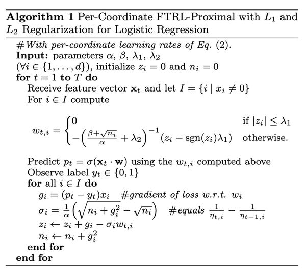
Observing the pseudocode, I noticed the main difference was swapping out the learning rate $\eta_t$ with $(\frac{\beta + \sqrt{n_i}}{\alpha} + \lambda_2)^{-1}$. It’s clear that the $\lambda_2$ is for L2-regularization, and my guess is that the extra $\alpha$ and $\beta$ hyperparameters help with numerical stability and convergence. The update rule for $z_i$ remained the same, and there’s a variable $n_i$ that keeps track of the running sum of squared gradients, which I assume is for memory efficency. The update rule for $\sigma_i$ is adapted for the new learning rate and we can confirm that it remained the same when you rewrite $\frac{1}{\eta_{t,i}} - \frac{1}{\eta_{t-1,i}}$ in terms of the adjusted $(\frac{\beta + \sqrt{n_i}}{\alpha} + \lambda_2)^{-1}$ learning rate.

keras implementation

The FTRL-Proximal algorithm has an implementation in Keras. After reading the paper, I decided to annotate the implementation to see what changes were made in code and how similar it is to the paper. The multi-line comments in green are my annotations.

def update_step(self, gradient, variable, learning_rate):
    """Update step given gradient and the associated model variable."""

    lr = ops.cast(learning_rate, variable.dtype)
    gradient = ops.cast(gradient, variable.dtype)

    accum = self._accumulators[self._get_variable_index(variable)]
    linear = self._linears[self._get_variable_index(variable)]

    lr_power = self.learning_rate_power
    l2_reg = self.l2_regularization_strength
    l2_reg = l2_reg + self.beta / (2.0 * lr)
    """
    lr = alpha
    
    l2_reg = lambda_2 + (beta / (2 * alpha)
    """

    grad_to_use = ops.add(
        gradient,
        ops.multiply(
            2 * self.l2_shrinkage_regularization_strength, variable
        ),
    ) # this is the shrinkage l2, directly apply on gradient -> 2 * lambda_2 * gradient
    new_accum = ops.add(accum, ops.square(gradient))
    """
    accum + g_squared
    accum = n
    n <- n + g_squared
    """
    self.assign_add(
        linear,
        ops.subtract(
            grad_to_use,
            ops.multiply(
                ops.divide(
                    ops.subtract(
                        ops.power(new_accum, -lr_power),
                        ops.power(accum, -lr_power),
                    ),
                    lr,
                ),
                variable,
            ),
        ),
    ) 
    """
    suppose lr_power = -1/2
    [ (n_i ^ 1/2 - n_{i-1} ^ 1/2) / lr ] * w_i
    
    variable = w_i
    linear = z_i (why did they write it this way...)
    
    z_i <- z_i + g - sigma * w
    """
    quadratic = ops.add(
        ops.divide(ops.power(new_accum, (-lr_power)), lr), 2 * l2_reg
    )
    """
    new_accum = n_i
    accum = n_{i-1}
    
    quadratic = 2 * l2_reg + (n_i ** 1/2) / alpha
    """
    
    linear_clipped = ops.clip(
        linear,
        -self.l1_regularization_strength,
        self.l1_regularization_strength,
    )
    """
    linear_clipped = sgn(z_i) * lambda_1
    """
    
    self.assign(
        variable,
        ops.divide(ops.subtract(linear_clipped, linear), quadratic),
    )
    """
    w_t = (sgn(z_i) * lambda_1 - z_i) / (2 * l2_reg + (n_i ** 1/2) / alpha)
    """
    self.assign(accum, new_accum)

jax implementation

The way I found out about this paper was because Optax, the optimization library for Jax, wanted an implementation of the FTRL-Proximal algorithm in their library. Unfortunately, the way Optax was designed assumes that gradient updates are additive, but the update rule for FTRL-Proximal is closed form and not with respect to the previous weights. The only workaround then is to compute $w_t$, update $z_t$, and compute $w_{t+1}$, and then take the difference $w_{t+1} - w_t$ as the gradient update, but this is inefficient. Check out my pull request for an interesting discussion about this and the lore of FTRL.

conclusion

Overall, really cool algorithm! I still think it’s pretty bonkers that Google used this to induce sparsity in billions of dimension feature vectors, the effectiveness of this algorithm at that scale makes it that much more impressive. I had my fair share of head-banging when I was working out the math (the paper gives only 4 equations total with no steps in between). Hope this annotated version helps anyone learning more about the algorithm!

references

[1] https://static.googleusercontent.com/media/research.google.com/en//pubs/archive/41159.pdf
[2] https://courses.cs.washington.edu/courses/cse599s/14sp/scribes/lecture3/lecture3.pdf